PyDLM ¶

Welcome to PyDLM, a flexible, user-friendly and rich functionality time series modeling library for python. This package implementes the Bayesian dynamic linear model (Harrison and West, 1999) for time series data analysis. Modeling and fitting is simple and easy with pydlm. Complex models can be constructed via simple operations:

# import dlm and its modeling components
from pydlm import dlm, trend, seasonality, dynamic, autoReg, longSeason
# randomly generate data
data = [0] * 100 + [3] * 100
# construct the base
myDLM = dlm(data)
# adding model components
# add a first-order trend (linear trending) with prior covariance 1.0
myDLM = myDLM + trend(1, name='lineTrend', w=1.0)
# add a 7 day seasonality with prior covariance 1.0
myDLM = myDLM + seasonality(7, name='7day', w=1.0)
# add a 3 step auto regression
myDLM = myDLM + autoReg(degree=3, data=data, name='ar3', w=1.0)
# show the added components
myDLM.ls()
# delete unwanted component
myDLM.delete('7day')
myDLM.ls()

Users can then analyze the data with the constructed model:

# fit forward filter
myDLM.fitForwardFilter()
# fit backward smoother
myDLM.fitBackwardSmoother()

and plot the results easily:

# plot the results
myDLM.plot()
# plot only the filtered results
myDLM.turnOff('smoothed plot')
myDLM.plot()
# plot in one figure
myDLM.turnOff('multiple plots')
myDLM.plot()

The three images show

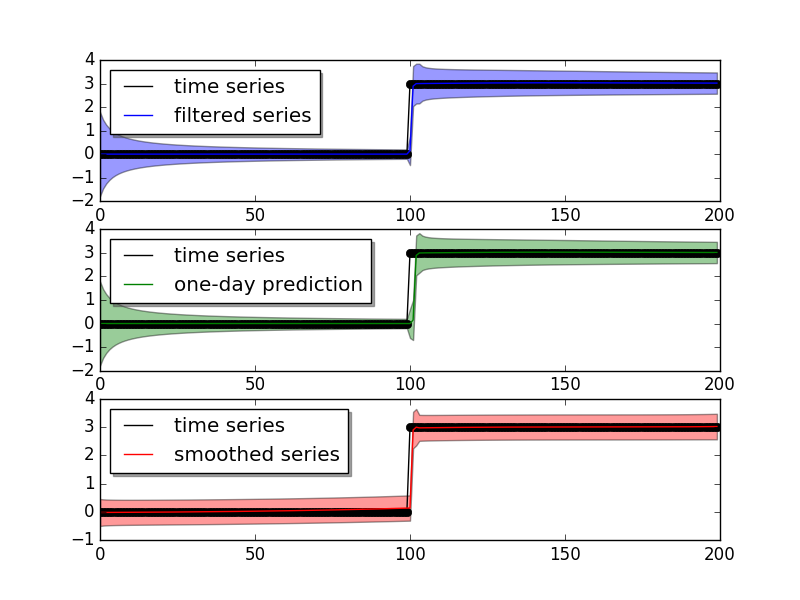
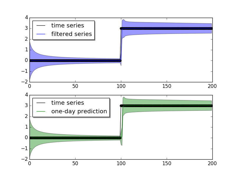
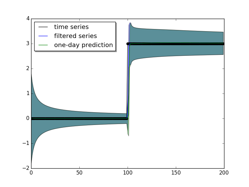
User can also plot the mean of a component (the time series value that attributed to this component):

# plot the component mean of 'ar3'
myDLM.turnOn('smoothed plot')
myDLM.turnOff('predict')
myDLM.plot(name='ar3')

and also the latent states for a given component:

# plot the latent states of the 'ar3'
myDLM.plotCoef(name='ar3')

which result in

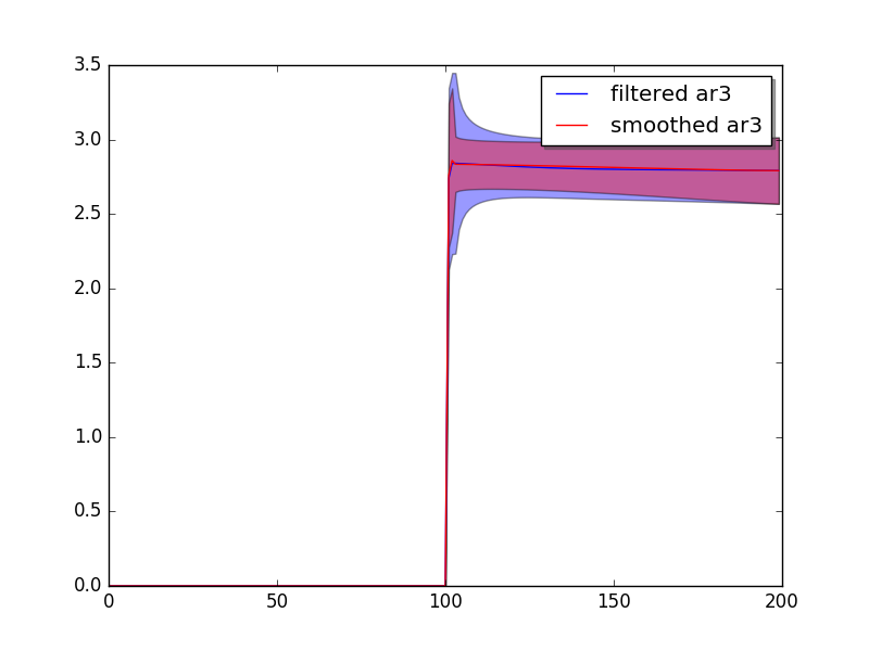
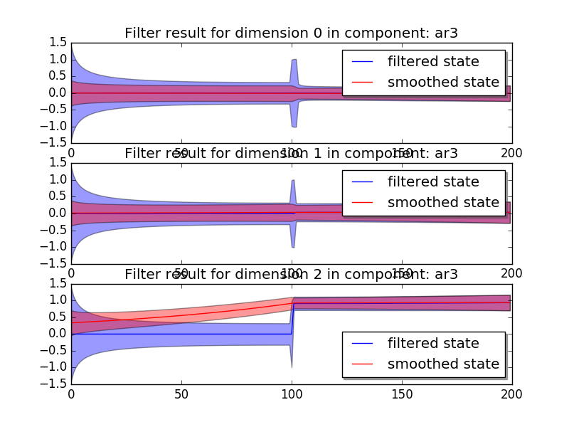
The ‘ar3’ has three latent states (today - 3, today - 2, today - 1), and the states are aligned in the order fo [today - 3, today - 2, today - 1], which means the current model attributes a lot of weight to the today - 1 latent state.

If users are unsatisfied with the model results, they can simply reconstruct the model and refit:

myDLM = myDLM + seasonality(4)
myDLM.ls()
myDLM.fit()

pydlm supports missing observations:

data = [1, 0, 0, 1, 0, 0, None, 0, 1, None, None, 0, 0]
myDLM = dlm(data) + trend(1, w=1.0)
myDLM.fit()  # fit() will fit both forward filter and backward smoother

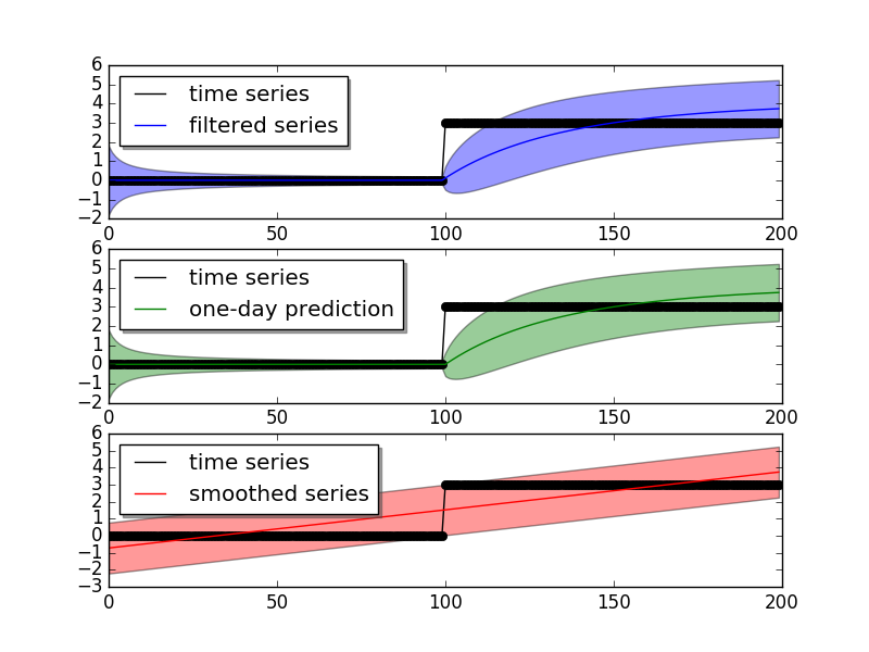
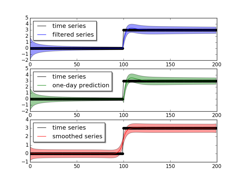
It also includes the discounting factor, which can be used to control how rapidly the model should adapt to the new data:

data = [0] * 100 + [3] * 100
myDLM = dlm(data) + trend(1, discount=1.0, w=1.0)
myDLM.fit()
myDLM.plot()

myDLM.delete('trend')
myDLM = myDLM + trend(1, discount=0.8, w=1.0)
myDLM.fit()
myDLM.plot()

The two different settings give different adaptiveness

The discounting factor can be auto-tuned by the modelTuner provided by the package:

from pydlm import modelTuner
myTuner = modelTuner(method='gradient_descent', loss='mse')
tunedDLM = myTuner.tune(myDLM, maxit=100)

and users can get the MSE of each model for performance comparison:

myDLM_mse = myDLM.getMSE()
tunedDLM.fit()
tunedDLM_mse = tunedDLM.getMSE()

The filtered results and latent states can be retrieved easily:

# get the filtered and smoothed results
filteredMean = myDLM.getMean(filterType='forwardFilter')
smoothedMean = myDLM.getMean(filterType='backwardSmoother')
filteredVar = myDLM.getVar(filterType='forwardFilter')
smoothedVar = myDLM.getVar(filterType='backwardSmoother')

filteredCI = myDLM.getInterval(filterType='forwardFilter')
smoothedCI = myDLM.getInterval(filterType='backwardSmoother')

# get the residual time series
residual = myDLM.getResidual(filterType='backwardSmoother')

# get the filtered and smoothed mean for a given component
filteredTrend = myDLM.getMean(filterType='forwardFilter', name='lineTrend')
smoothedTrend = myDLM.getMean(filterType='backwardSmoother', name='lineTrend')

# get the latent states
allStates = myDLM.getLatentState(filterType='forwardFilter')
trendStates = myDLM.getLatentState(filterType='forwardFilter', name='lineTrend')

For online updates:

myDLM = dlm([]) + trend(1) + seasonality(7)
for t in range(0, len(data)):
...     myDLM.append([data[t]])
...     myDLM.fitForwardFilter()
filteredObs = myDLM.getFilteredObs()

PyDLM¶

Documentation¶

PyDLM ¶